Building a QPU simulator in Julia - Part 4
Recall that Deutsch’s algorithm can be represented by the following circuit:
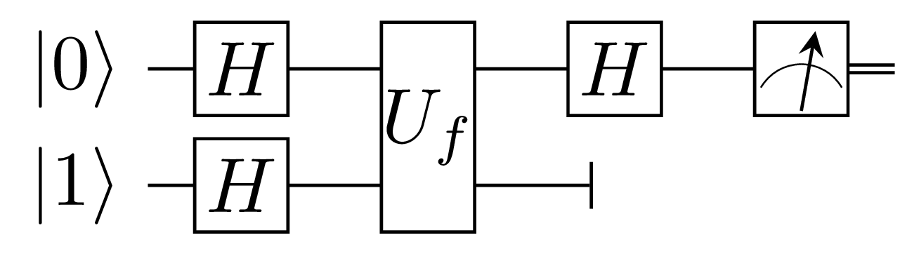
We want something like this, remembering that Julia is 1-index based:
deutch(Uf) = register(ZERO, ONE) |>
                gate(H, H) |>
                gate(Uf) |>
                gate(H, eye) |>
                measure(1)
We already have most of the machinery to make this work. We need an overloaded register function to create a register with the given states. This is straightforward and very similar to the gate function we defined in the last post.
register(x...) = foldl(kron, x)
Next a pipeable measure function that takes the bit k that we want to measure (1-indexed).
measure(n, k) = (qubits) -> measure!(n, k, qubits)[1][k]
To avoid having to pass in the size of the register, we can calculate it from the length of the qubits vector. We know that the length, $l$, of the vector is $l=2^{n}$ so $n=\lfloor log_{2}(l) \rfloor$. In code that becomes:
size(qubits) = Int(floor(log2(length(qubits))))
measure(k) = (qubits) -> measure!(size(qubits), k, qubits)[1][k]
All that remains is to define the oracle \(U_{f}\). For 2-bit inputs there are four possible functions:
| $x$ | $f_1(x)=0$ | $f_2(x)=x$ | $f_3(x)=\bar{x}$ | $f_4(x)=1$ | |
|---|---|---|---|---|---|
| 0 | 0 | 0 | 1 | 1 | |
| 1 | 0 | 1 | 0 | 1 | |
| constant | balanced | balanced | constant |
The transformation we need for the oracle is from $\ket{x}\ket{y}$ to $\ket{x}\ket{y⊕f(x)}$ which we can write out explicitly.
| $x$ $y$ | $y⊕f_1(x)$ | $y⊕f_2(x)$ | $y⊕f_3(x)$ | $y⊕f_4(x)$ | |
|---|---|---|---|---|---|
| 0 0 | 0 | 0 | 1 | 1 | |
| 0 1 | 1 | 1 | 0 | 0 | |
| 1 0 | 0 | 1 | 0 | 1 | |
| 1 1 | 1 | 0 | 1 | 0 |
Reading off the columns we have:
| $y⊕f_1(x)$ | y |
I |
| $y⊕f_2(x)$ | x?~y:y |
Controlled NOT |
| $y⊕f_3(x)$ | y?~x:x |
Reversed Controlled NOT |
| $y⊕f_4(x)$ | ~y |
NOT |
The matrices that do those transformations can be written as direct sums,which is available in Julia as the blockdiag function:
Uf1 = blockdiag(eye, eye) # I
Uf2 = blockdiag(eye, NOT) # C-NOT
Uf3 = blockdiag(NOT, eye) # Reversed C-NOT
Uf4 = blockdiag(NOT, NOT) # NOT
If the function, $f$, is balanced then the measurement will always be true, if constant then the measurement will always be false. Let’s evaluate them all together:
julia> map(deutch, [Uf1, Uf2, Uf3, Uf4])
Bool[false, true, true, false]
We can see that this is exactly the result we expect.
Extending to multiple bits, the generalised quantum circuit in this case is:
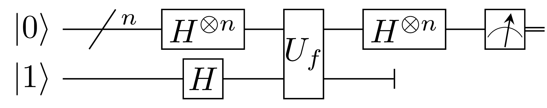
This is known as the Deutsch-Jozsa algorithm. The wikipedia article has much more information about how this works. In our Julia DSL we can easily extend to 2-bit functions:
deutchJosza(Uf) = register(ZERO, ZERO, ONE) |>
                gate(H, H, H) |>
                gate(Uf) |>
                gate(H, H, eye) |>
                measure(1:2)
We could determine the transformations $U_f$ like before by writing them out explicitly but new we have 8 possible permutations. Rather than writing them out let’s write a function to do it for us:
oracle(n::Int, f) = begin
    perm = Dict{Int,Int}()
    for x in 0:2^n-1
        for y in 0:1
            xy = (x << n) + y      # |x>|y>
            fxy = y ⊻ f(x)         # |y⊕f(x)>
            xfxy = (x << n) + fxy  # |x>|y⊕f(x)>
            perm[xy+1] = xfxy+1    # mapping (1-index based)
        end
    end
    permmat(map((it) -> perm[it], 1:2^(n+1)))
end

permmat(π) = sparse(1:length(π), π, 1)
This function goes through the $2^n$ possible values of $\ket{x}$ and the two possible values of $\ket{y} \in (0,1)$ and builds a transformation table, perm, of the values $\ket{x}\ket{y}$ to $\ket{x}\ket{y⊕f(x)}$. This table is then used to create a (sparse) permutation matrix for the transformation, e.g. $U_f$. This is a very brutish way of doing it but it gets the job done.
Finally we can run the algorithm and check it works
deutchJosza(Uf) = register(ZERO, ZERO, ONE) |>
                gate(H, H, H) |>
                gate(Uf) |>
                gate(H, H, eye) |>
                measure(1:2) |>
                (y) -> reinterpret(Int, y.chunks)[1] != 0


Uf1 = oracle(2, 1, (x, y) -> y ⊻ 0)
Uf2 = oracle(2, 1, (x, y) -> y ⊻ (x & 1))
Uf3 = oracle(2, 1, (x, y) -> y ⊻ (x & 1 ⊻ 1))
Uf4 = oracle(2, 1, (x, y) -> y ⊻ 1)

@test map(deutchJosza, [Uf1, Uf2, Uf3, Uf4]) == [false, true, true, false]
The line reinterpret(Int, y.chunks)[1] != 0 converts the binary result to an integer and checks if it’s different from 0.
That’s the Deutch-Jozsa algorithm complete. Next one will be Grover’s algorithm, then Simon’s algorithm before we get into the QFT and finally Shor’s famous factoring algorithm.